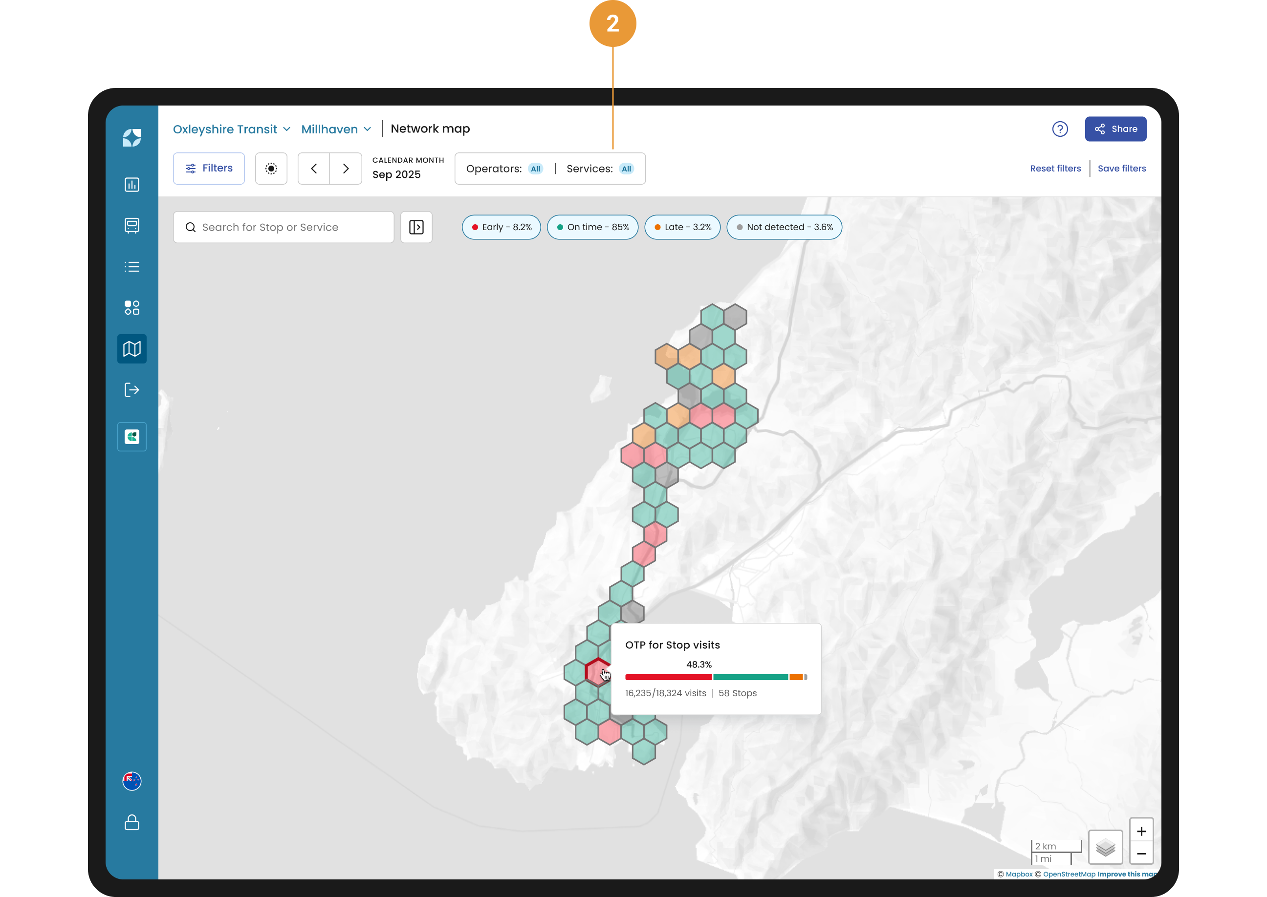
The on-time performance (OTP) overlay helps users see the signal in the noise, compare areas, and guide smarter decisions. An hexbin map, also known as a hexagonal bin map, divides a spatial area into hexagons and uses colour to represent data aggregated within each hexagon.
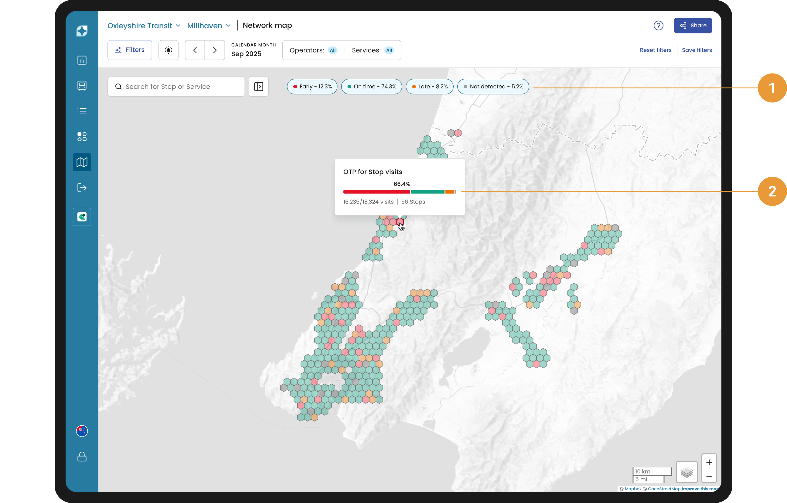
By default, Early on time performance is selected (1). Toggle these chips on/off to allow you to quickly identify where the problems are in the network (early, late, not detected) so that a deeper exploration can start. Hover over hexbins to view a summary of performance for stops in that hexbin (2).
Please refer to the FAQs for more information on the categories of on time performance.
How OTP is visualised
-
OTP appears as hexbins on the map, coloured by their corresponding category (Red = Early; Green = On time; Orange = Late; Grey = Not detected)
-
Each hexbin contains a number of stops which determines the hexbin colour. Each hexbin is coloured by the predominant Early, On-time & Late (EOL)* of the stops inside the hexbin.
-
Single and multiple selection of EOL chips, renders different colours.
-
When multiple EOL chips are selected, the map shows solid colours, each colour corresponding to the selected category. The colour of the hexbin represents the EOL with the greatest value.
-
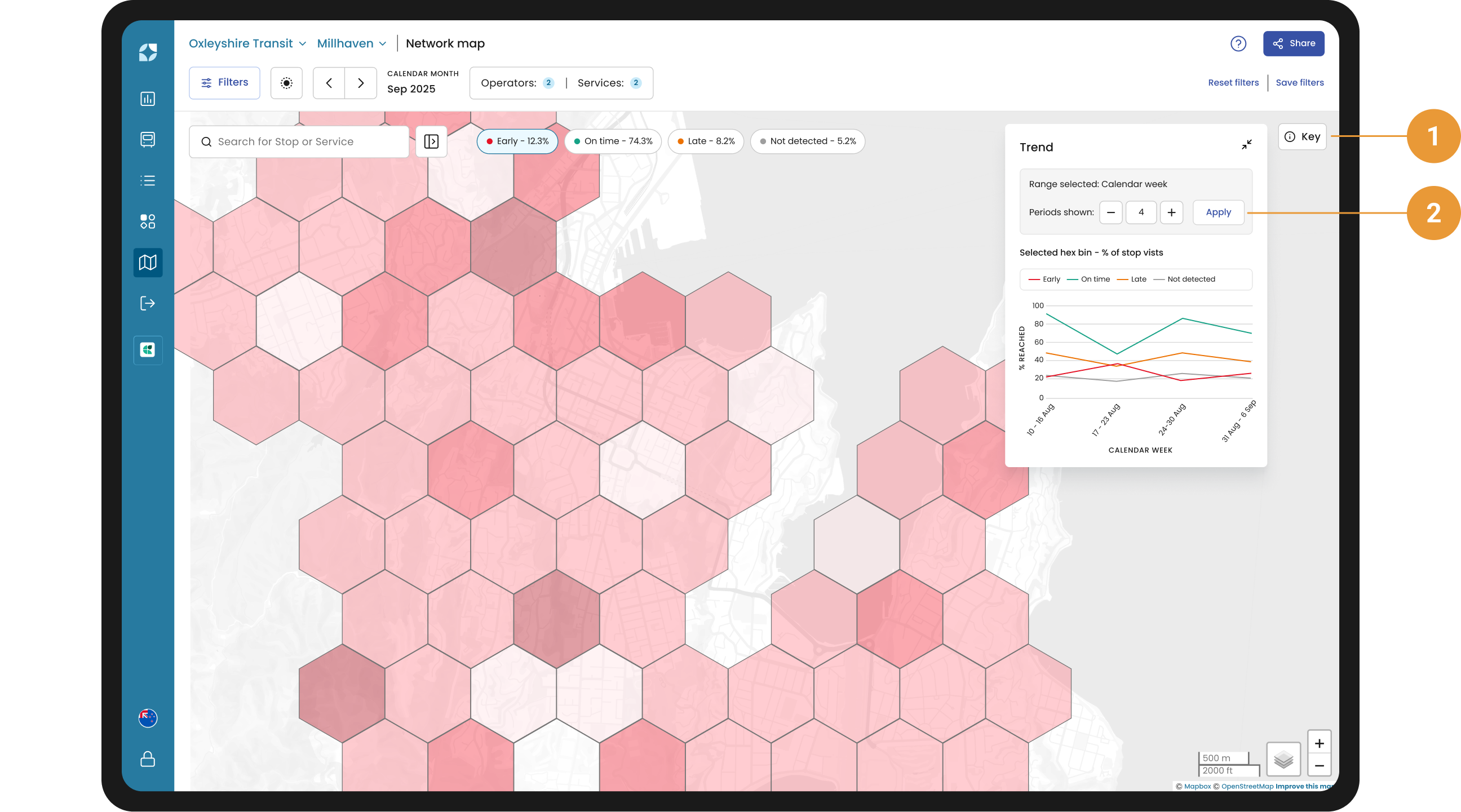
When a single EOL chip is selected, the map shows a single colour dispersed through a range of values, from lighter colour representing lower numbers, to darker colour representing larger numbers. The key describes what each colour shade represents.
-
*Please refer to the FAQs for more information on how EOL is defined.
OTP Trends
By default, the network-wide trend for early on-time performance is shown next to the Key in the top right of the Network map (1). Collapse it the same way you'd collapse the Key. Toggle the EOL chips on/off to see the trend for on-time, late and not detected. Click on either a hexbin, stop or service to view their performance trends.
The trend allows you to visualise the EOL performance over time. It reflects whatever date range and exclusions you have applied in the filter hub. For example, choose Calendar month and the trend will plot monthly performance, choose Calendar week and it will plot weekly performance.
Choose how far back you view by adjusting the periods shown (2), either with the plus and minus buttons, or type a number directly, and click Apply.
Interactive Features
-
Hover over a hexbin: Get an instant pop-up showing key information, including:
-
Number of stops inside the hexbin.
-
Number of actual visits compared to the scheduled visits to the stops.
-
OTP bar showing the aggregation of all the stops' on-time performance percentages.
-
-
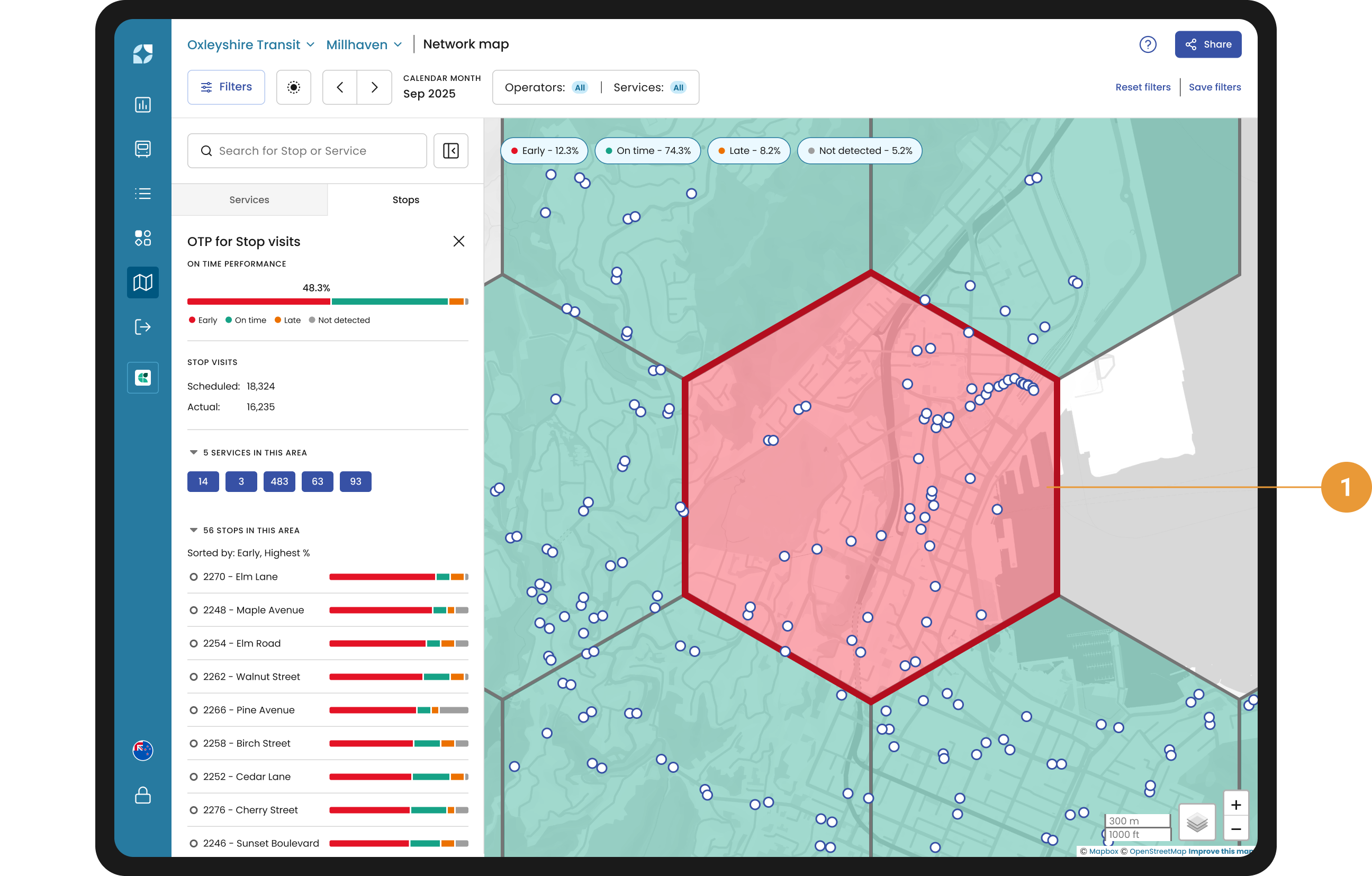
Click on a hexbin: Clicking on a hexbin opens a side panel (1), that provides a detailed breakdown of the on-time performance for all stops within that hexbin. This helps you move from high-level hotspot detection to stop-level diagnosis in just one click. The side panel includes:
-
Aggregated OTP bar for the selected hexbin, showing the overall percentage breakdown of Early, On time, Late and Not detected stop visits.
-
Scheduled vs. actual stop visits count, giving you visibility into data completeness and reliability.
-
A list of stops within the selected hexbin, sorted by the highest percentage of the dominant EOL category (e.g. sorted by Early %, if early is the leading issue
-
Additional Tips
-
You can filter the visualisation to a number of services (2). In this case, the hexbins will only be shown covering the stops used for the selected services.